For the PDC summer course Introduction to High Performance Computing, Martin Biel and I wrote a BVH builder in CUDA based on a HPG paper by Tero Karras. The work uses Morton codes, 3D space-filling curves, to construct the bounding volume hierarchy very quickly on the GPU.

The main idea is to represent the BVH as a binary search tree, where each internal node forms an axis-aligned bounding box around its children nodes. The leaf nodes are the bounding volumes around each individual triangle. To construct the tree the triangles are first sorted according to their spatial locality, and then converted into a binary tree which is finally traversed to construct the intermediate bounding volumes in the hierarchy.

Morton codes constitute a mapping between 3D coordinates and 1D coordinates that preserves the spatial locality. The Morton code of a given 3D coordinate is determined by interleaving the bit representation of each xyz coordinate into one binary number. A consequence of this representation is that a sorted list of Morton codes naturally form a data structure where adjacent entries are in close proximity in 3D space. The sorted list can be used to construct a binary search tree, which will form the basis of the bounding volume hierarchy.

Two adjacent Morton codes form the children of one internal tree node. Four adjacent Morton codes form a sub-tree of two internal nodes corresponding to two adjacent pairs, which in turn form the children of another internal node. The construction of the tree is made by splitting the sorted list of Morton codes recursively. If the split is made at the point where the highest bit differs between codes at the left and right side of the split, then a binary structure that preserves the locality is obtained. Each internal node in the tree is defined by the bit prefix shared by all of its children nodes. Consequently, the resulting structure is a binary radix tree.

Here is a visualization of the hierarchy on the Stanford Dragon model.

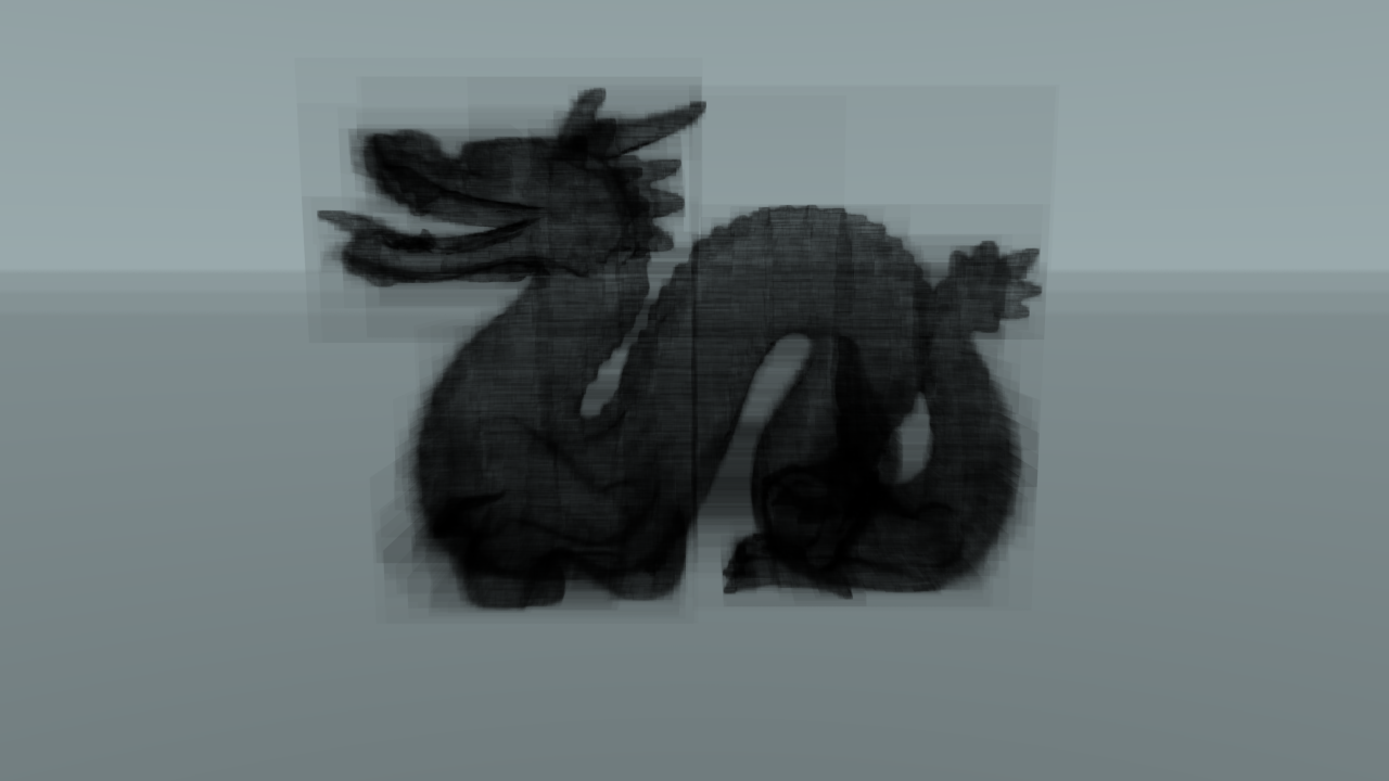
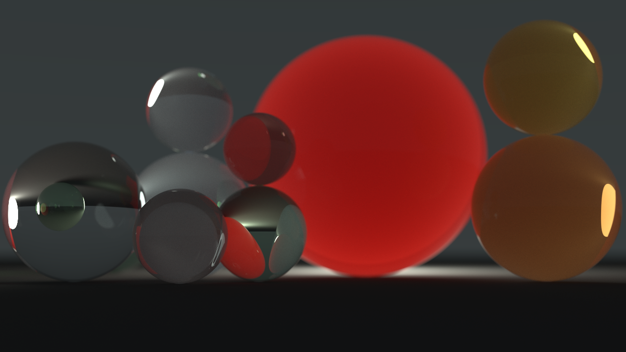
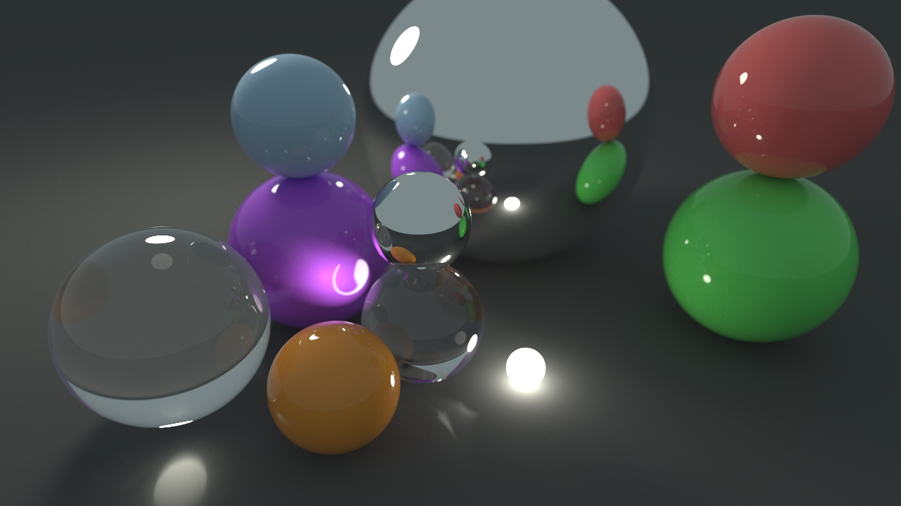
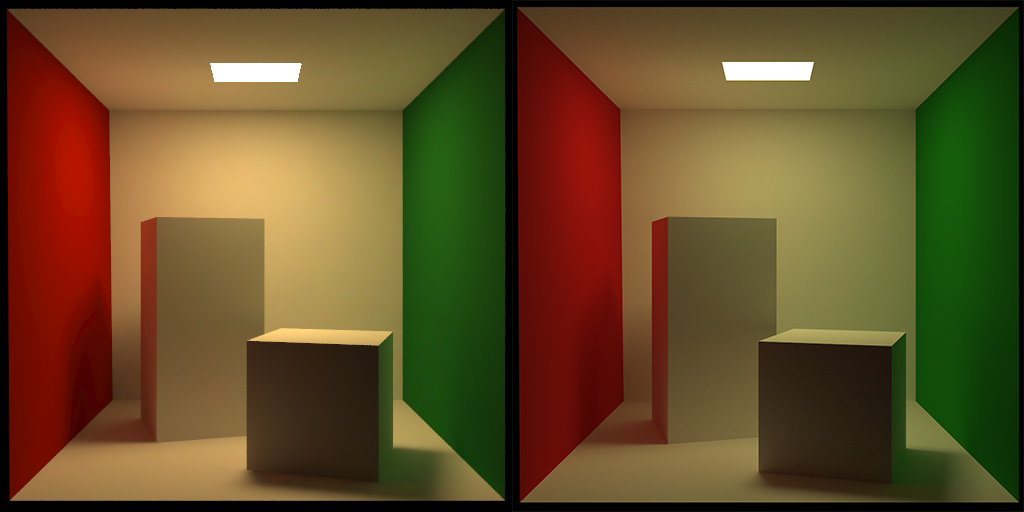
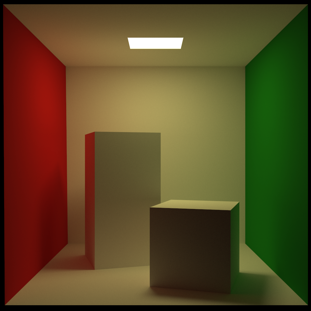
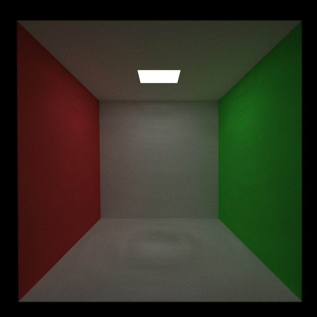
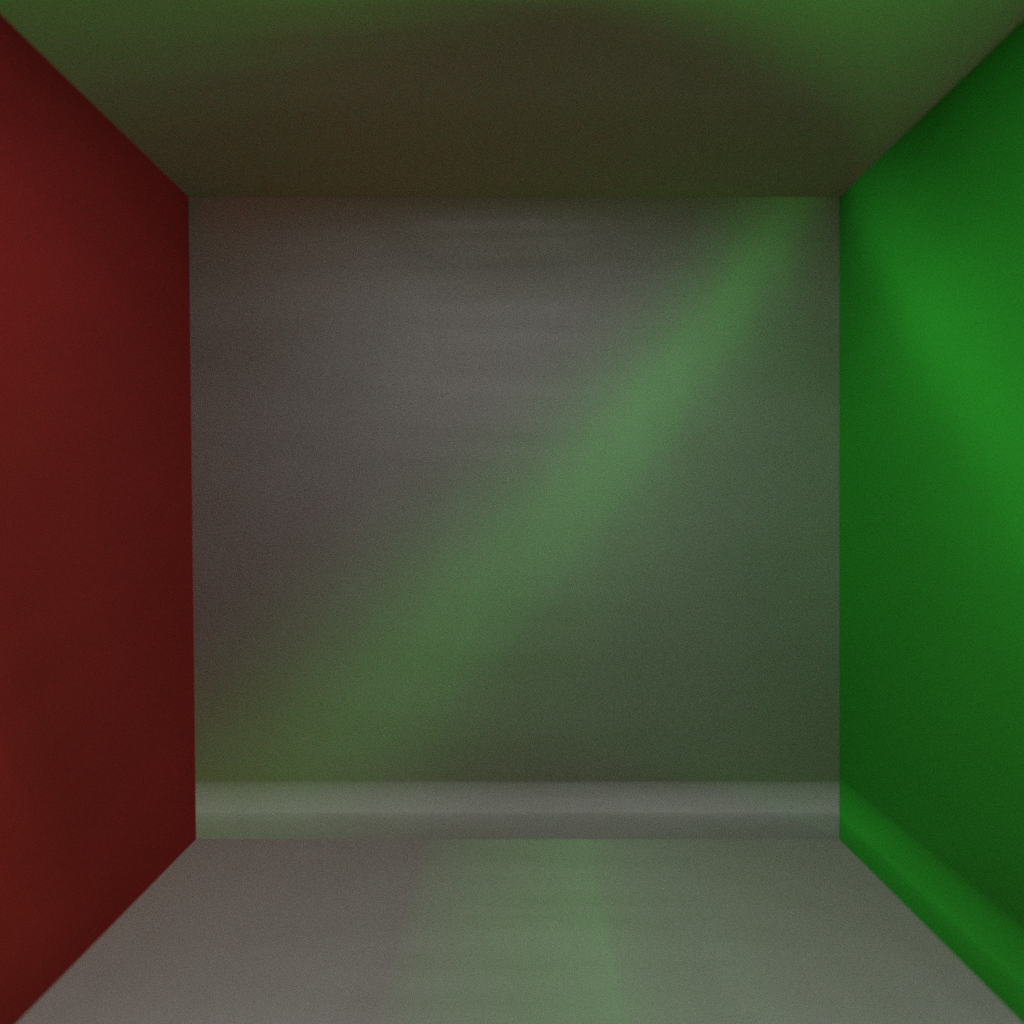
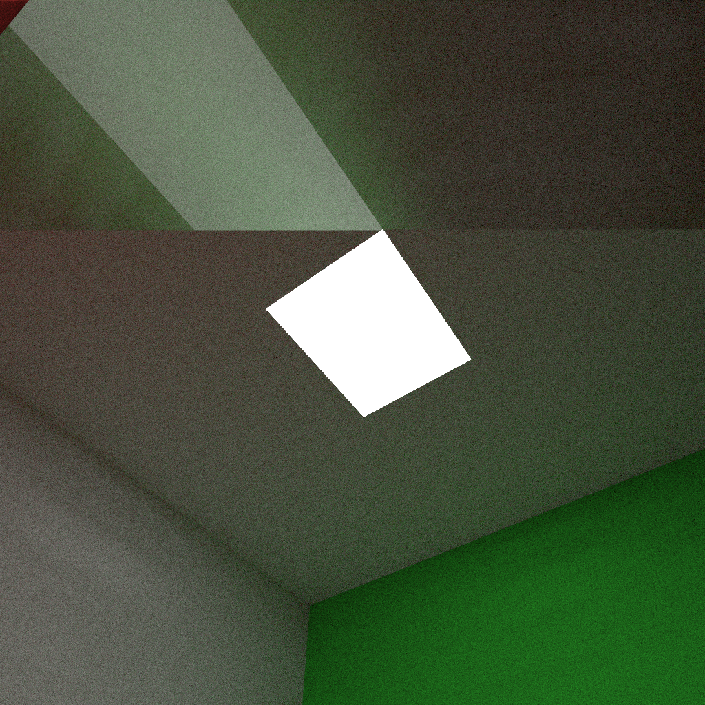
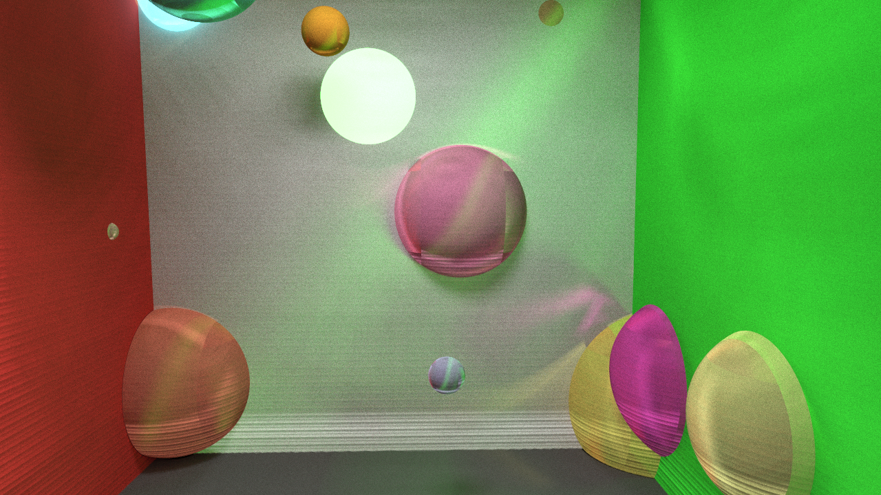
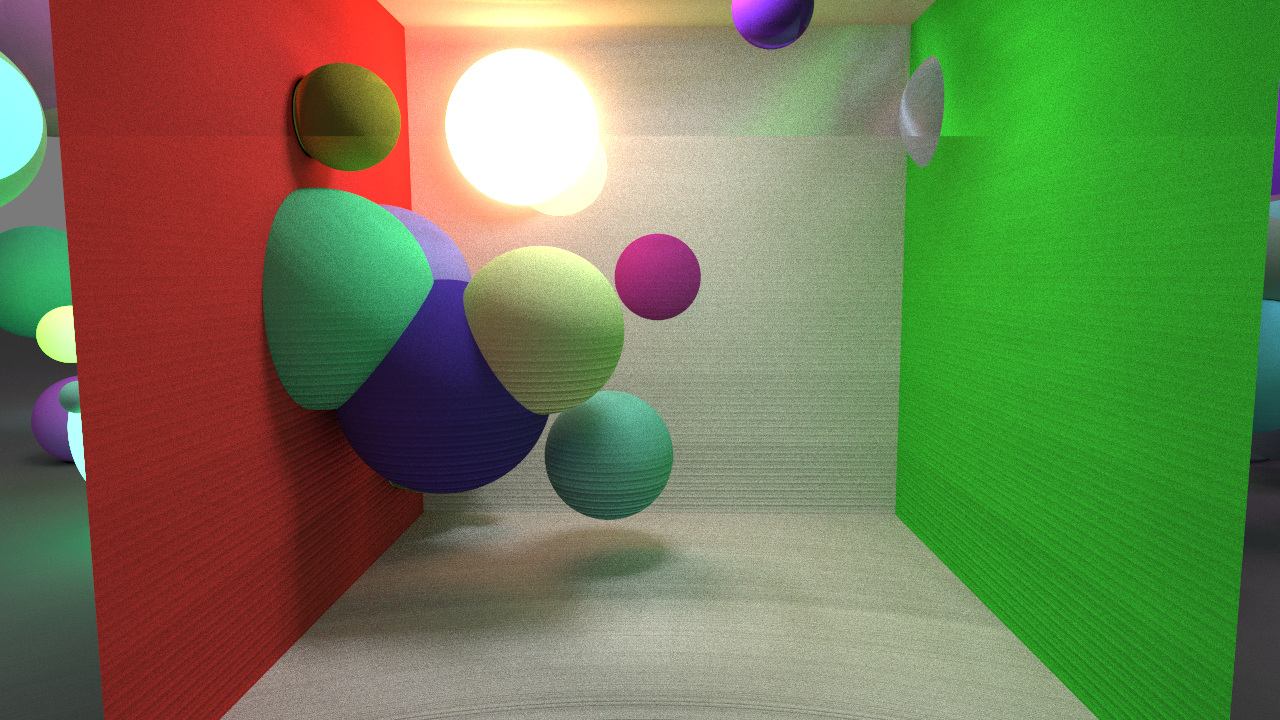
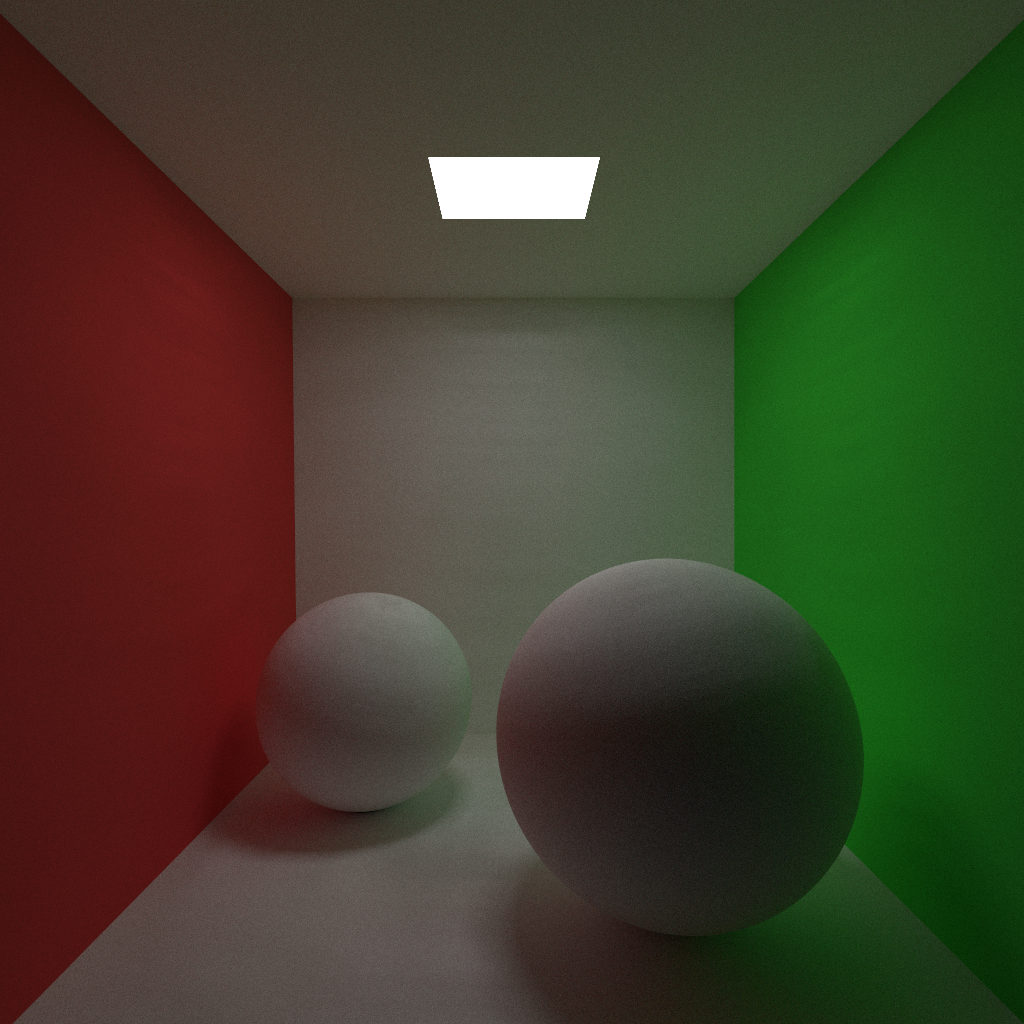
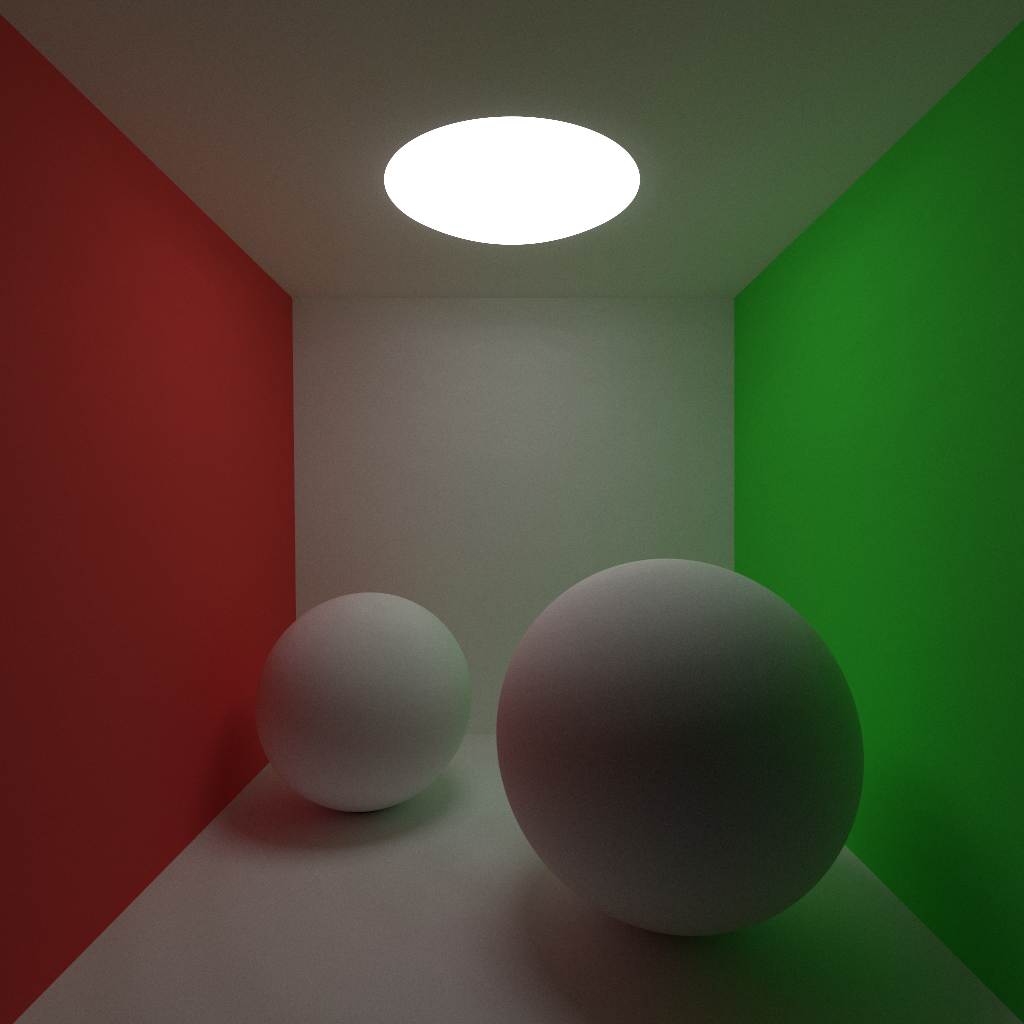
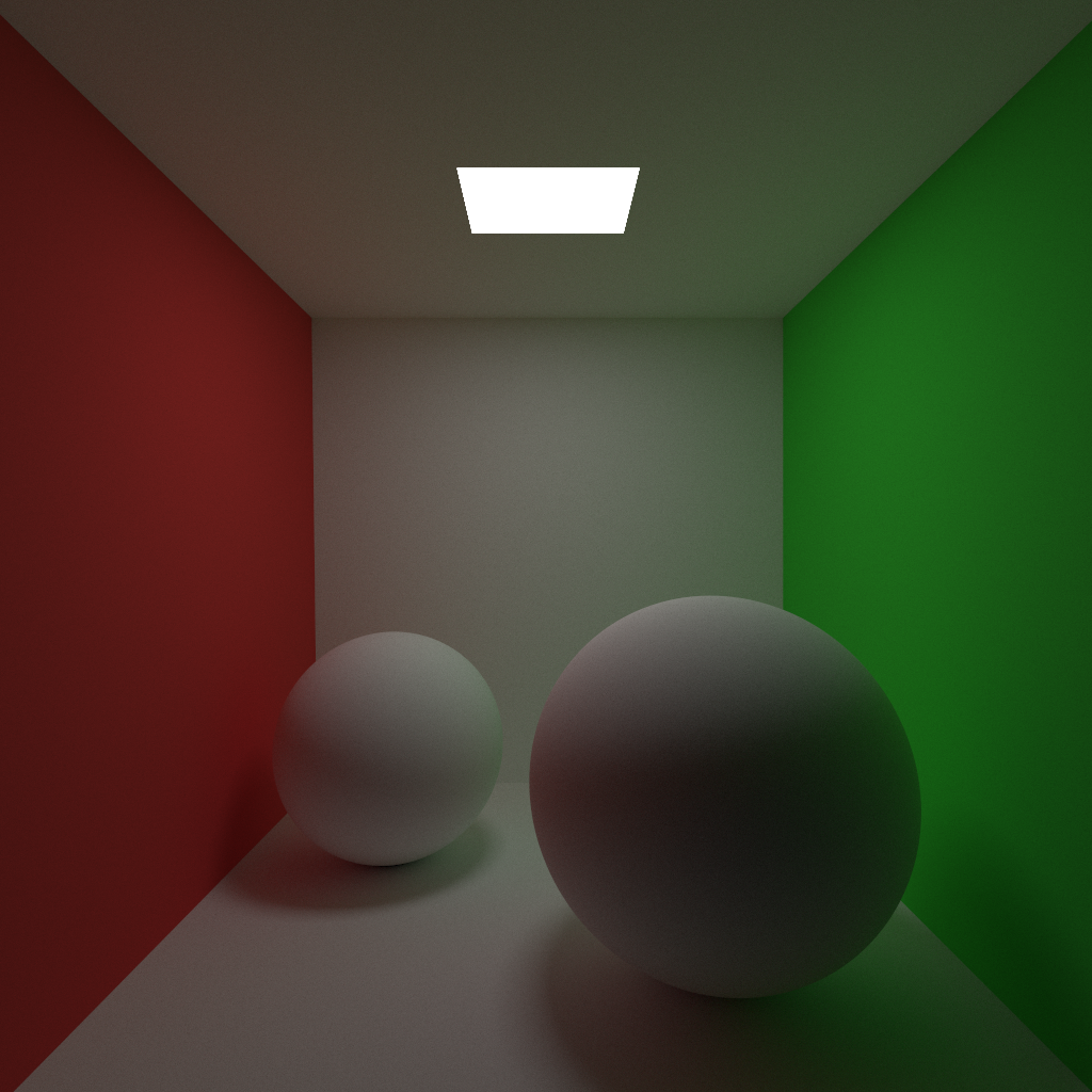
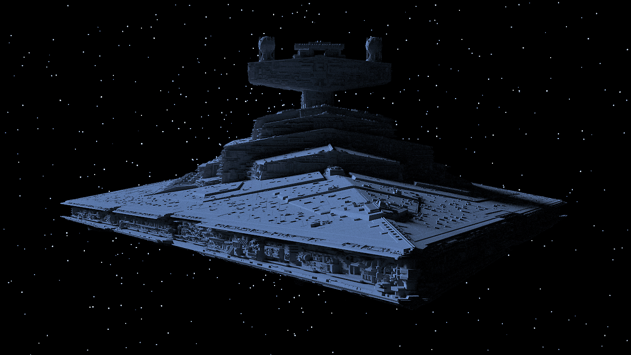
There are lots of technicalities in how to avoid recursion on the GPU and prevent race conditions between GPU threads when constructing the BVH from the radix tree, as well as how to traverse the tree on the GPU once it is built. I advise anyone interested in the details to read the paper, as well as the follow-up paper by Tero Karras and Timo Aila on how to improve trees build by this method. The BVH introduced here is not necessarily superior to a BVH built according to SAH or a similar heuristic, but since it is generated on the GPU it builds hierarchies very quickly, allowing it to be used in interactive applications such as games that require fast BVH generation and intersection tests for things such as collisions. In short, the implementation allows me to generate a BVH for a scene in the matter of milliseconds, and as with any acceleration structure the number of intersection tests is reduced dramatically. To summarize, below are some images rendered in my CUDA path tracer that would have been very time consuming if not for the implementation of a BVH.

A model of a Star Destroyer from my favourite franchise Star Wars. I haven’t implemented texture mapping yet so it is missing some detail, looking a bit dull and perhaps not doing the thing from the films justice. The stars are modeled by small, bright spherical light sources at a randomized distance from the model center. The model is lit by a larger sun-like object from the side.

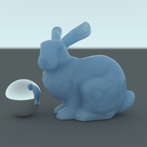
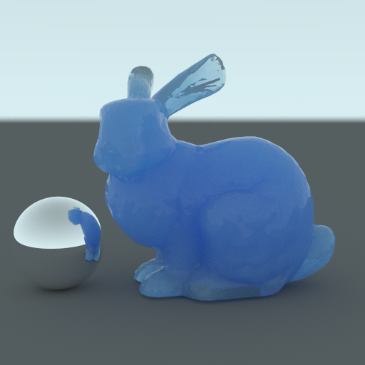
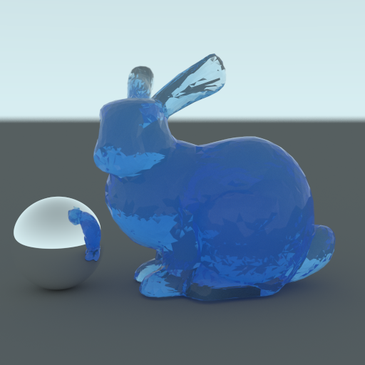
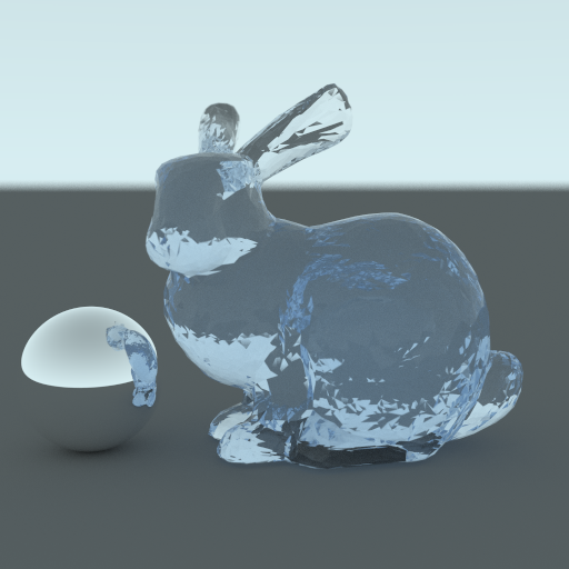
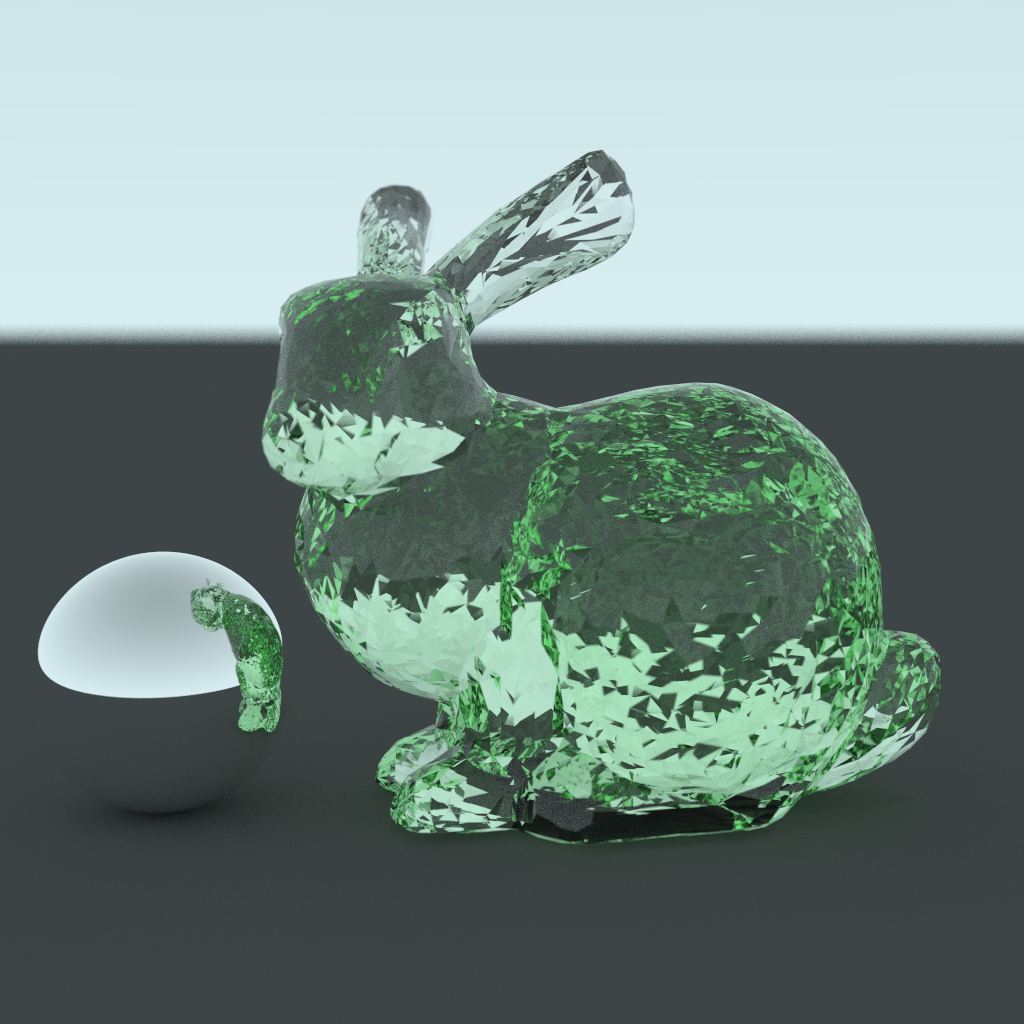
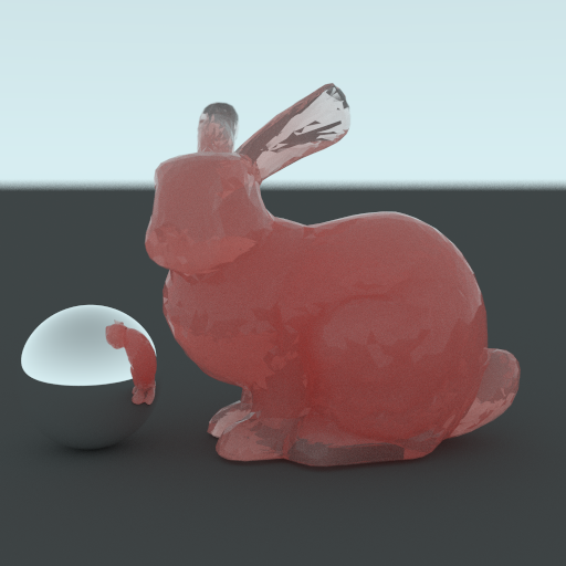
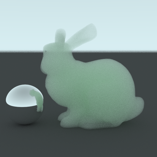
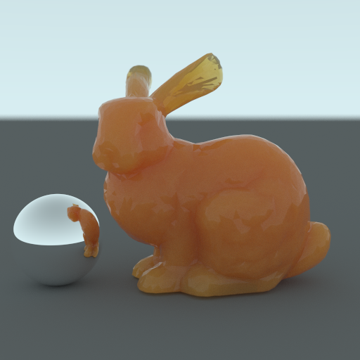
And here is the model currently featuring the front page of the blog. It’s the well known Stanford Bunny and Dragon rendered with the brute-force subsurface scattering implementation of my renderer.

It’s been a long time since I made an update here on the blog. The blog has moved from its old home to this page hosted on GitHub, and has received a new theme. As I’m getting closer to finishing up my Master’s thesis, I’ll have more time to work on hobby projects. My plan is to start working on a CPU-based renderer using some solid frameworks such as Embree and TBB at it’s core, allowing me to play around with fluid, smoke and fire simulations, rendering algorithms and some reinforcement learning stuff I’ve been interested in lately.

I’ve spent the year of 2017 working mostly on the thesis which is supervised by Jaakko Lehtinen. The thesis work is related to the very exciting field of gradient-domain light transport, and I’ve been working specifically with the gradient-domain path tracing method. Markus Kettunen, the main author of the paper, has been advising me for the thesis project. It’s truly been a blessing to work close to these two brilliant researchers as well as others in the Aalto graphics team.

In the fall semester of 2016 leading up to my Erasmus exchange at Aalto university I was spending most of my time finishing math classes, but my good friend Martin Biel and I did take a summer course at PDC Center for High Performance Computing in which we got to do a project in parallel programming. We decided to build a GPU BVH builder in CUDA which I will write about in my next blog post.

The renderer now features isotropic Monte Carlo subsurface scattering. The implementation is not limited to subsurface scattering but works as a general volumetric participating media system. To show it in images by rendering smoke or something similar would require more 3D modelling however. 

The implementation uses the reduced scattering coefficient and the absorption coefficient to sample a scattering distance and direction and compute the absorption. A higher scattering coefficient results in less transparency in the material, and the color of the material is determined by the absorption. Below are 4 renderings of the Stanford bunny at reduced scattering coefficients of 64, 16, 4 and 1, respectively. In the rightmost picture, the absorption coefficient has been reduced as well, giving off the appearance of blue-tinted glass. Notice also how the material appears clearer in areas such as the ears and tail where the model is not as thick.

The material absorption is computed using the Beer-Lambert law. When the scattering coefficient is high, the distance traveled by the light is low which means that the transmission from the Beer-Lambert law is going to be higher for a given absorption coefficient. This is why the blue color appears darker and darker as the scattering coefficient is reduced, except in the case where the absorption coefficient has been reduced.

This method of computing volumetric scattering is brute-force and therefore takes a lot longer to converge than for ideally specular, transmissive and diffuse materials. When rendering these images I used a maximum number of ray bounces of 40, which means that it will take a long time for many rays before they terminate. This is necessary in order to capture the subsurface scattering phenomenon well, but means that the time spend per iteration is longer. The fact that I don’t have an acceleration structure in place yet makes things even worse, as I currently check for intersections with the over 4k triangles of the bunny model in a serial fashion. Nevertheless, when rendering images like this at a resolution of 512x512 pixels, the engine spends around half a second per iteration, which is fast enough to show some of the implemented rendering models if not quite fast enough for interactive use.

Below are some subsurface scattering pictures and more bunnies, including one where the index of refraction is set to be lower than that of air, resulting in 100% transmission rate and a smoke-like bunny.

​

This will be the last contribution to the renderer for this project, though I will continue developing it in my free time to learn more. Below is a list of some of the immediate system-related concerns I aim to fix in the renderer, as well as graphics features I would like to add incrementally.

• Parallel BVH construction/traversal
• Memory manager class for CUDA
• Separate ray tracing and BSDF evaluation into separate kernels
• Proper system for material modeling, very hardcoded at the moment
• Robust and flexible scene/mesh loading
• Replace legacy OpenGL calls with a modern implementation
• Wireframe/Lightweight rendering mode
• Dithering
• Microfacet modelling
• Anisotropic subsurface scattering
• Texture/Normal/Displacement/Environment mapping
• Bidirectional Path Tracing
• Metropolis Light Transport
• …

I have implemented pure reflective and transmissive materials into the renderer as well as glossy materials, using the Fresnel equations to compute the reflectance R and transmittance T. When a ray intersects a primitive in the scene, the reflection and transmission directions are computed from the incident direction, the surface normal and the refractive indices of the mediums on each side of the boundary. For specularly transmissive materials, one approach is to trace both the reflected and the refracted ray through the scene. Another approach that gives the same expected value for the computed radiance is to take a specular sample with probability equal to the computed Fresnel reflectance. This approach is known as russian roulette and is commonly used in various statistical scenarios. We sample a uniform random number and if this number is less than the computed R, we take a reflected ray sample. Otherwise we take a transmitted ray sample If the material is transmissive or a diffuse sample if it is not.

Below are a few renders showing these effects. The glossy materials are have reflected and diffuse samples, the mirror materials are purely reflective, and the transparent materials have reflected and transmitted samples.

The Lambertian diffuse samples, sampled by randomizing a cosine-weighted direction in the hemisphere, is actually just an approximation to the more general phenomenon of subsurface scattering, where light enters a material and is scattered around and absorbed before it exits the material. Such a phenomenon is modelled by the bidirectional subsurface reflectance distribution functions (BSSRDF) that encapsulates these volumetric scattering properties. When a material is modelled by a physically based BSSRDF that expresses low tranmissive properties and when the refractive index between the adjacent media is similar, the material will exhibit a diffuse appearance that the Lambertian model is trying to mimic. The next blog post will be about an attempt at implementing this into the renderer.

Before moving on to implementing more materials and a bounding volume hierarchy for triangle meshes, not to mention cleaning up the triangle mesh implementation itself, I decided to render the original Cornell box scene properly. I took the measured data for the scene and put it in the scene specification of my renderer. The positions of the camera and all the triangle vertices correspond completely with the data, but getting the correct color values for the scene components and the roof light was done by trying to come as close to the reference picture as possible. The field of view of the camera is also not completely correct. Below is a comparison between my rendering and the reference image. Can you see which is which?

The colors match quite well but there’s some tweaking to be done to get it completely right. Below is the rendering in its full resolution. The image was rendered with 65k samples per pixel with a maximum ray depth of 10, each pass taking around 82ms to complete, resulting in a total rendering time of approximately 1,5 hours. The convergence was very slow due to the relatively dim lighting and my hope is to implement more sophisticated rendering methods such as bidirectional path tracing or metropolis light transport in the future to improve the sampling.

This post will be about some errors I remedied this week that had to do with bad random number generation. I realized there was something wrong with the rendering when I approached some scene objects closer than usual. I’m not sure why this is, but after stepping inside the Cornell box I had set up for the scene, artefacts popped up that hadn’t been there earlier. Below are some pictures displaying these errors.

I tried to change the hemisphere sampling kernel without any success, after which I started playing around with the seed that’s passed to the random number generators in the kernels. After each ray bounce, I was not reseeding the random number generator based on the ray depth, causing the seed to be the same at each bounce for the individual rays. I changed the seed to take the ray depth into account, after which I also started seeding everything form the system time in milliseconds resulting in a different seed each time the scene is reset, for instance when the camera is moved.

After having done this the renderings of the Cornell box scene still exhibited strong bias like in the upper leftmost picture above, shown in the leftmost picture below. I tried increasing the maximum ray depth, thinking that this might have been the source of the bias, but it barely changed anything. Switching to a sphere light instead of the square light changed the bias slightly as can be seen in the middle picture below, but that’s obviously not an acceptable solution since a rendering system ideally shouldn’t have to take such details of the scene into account.

Having looked around the web for similar projects I know that some - like me up until this point - generate random numbers using the cuRAND library, and some use the thrust library. I tried switching the cuRAND implementation for a corresponding implementation using the thrust library and voilá, the bias was gone, shown in the rightmost image below. I’m sure there was something wrong in the way I implemented the cuRAND function calls and fixing this would probably have remedied the problem. That would have required me to identify why the implementation wasn’t working however and as I am also using thrust for stream compaction I will stick to this method for random number generation as well.

While this error was incredibly annoying to chase down, it’s interesting in retrospect to see the effects of bad random number generation. My first thought when seeing the errors at the top of this post was certainly not that it was the RNG seeding that caused it. I spent a lot of time going through the camera implementation to see if it was the camera movement causing it, or if there was any self-intersection going on in the tracing kernels, so this has been very educational.